In this tutorial, we will predict the geolocation of IoT devices, based on the metadata of the messages they emit. The messages are received by stations belonging to the 0G network deployed by Sigfox.

The guidelines are taken from a course project at Télécom Paris, for an IoT course given by Sigfox.

The goal of the project is to manipulate data coming from IoT devices (with issues like faulty data) and to predict coordinates (latitudes and longitudes, which are two different labels to predict, but work together).

The complete code is available on the GitHub repository of the project.

Imports

import seaborn as sns
import numpy as np
import pandas as pd
import matplotlib.pyplot as plt
from geopy.distance import vincenty

from sklearn.metrics import accuracy_score
from sklearn.preprocessing import OneHotEncoder
from sklearn.model_selection import train_test_split, cross_val_predict
from sklearn.ensemble import RandomForestRegressor, ExtraTreesRegressor

1. Load and explore data

1.1. Data loading

# load train data
df_mess_train = pd.read_csv('./data/mess_train_list.csv') # train set
pos_train = pd.read_csv('./data/pos_train_list.csv') # position associated to train set

print("Number of observations in messages: ", df_mess_train.shape[0])
print("Number of observations in positions:", pos_train.shape[0])

Number of observations in messages:  39250
Number of observations in positions: 39250

1.2. Data description

Table messages

This table contains messages emitted by devices and received by stations. Some messages appear multiple times, because they are received by multiple stations. We will try to predict, from this information, the location of the device that emitted the messages.

df_mess_train.head()

	messid	bsid	did	nseq	rssi	time_ux	bs_lat	bs_lng
0	573bf1d9864fce1a9af8c5c9	2841	473335.0	0.5	-121.5	1.463546e+12	39.617794	-104.954917
1	573bf1d9864fce1a9af8c5c9	3526	473335.0	2.0	-125.0	1.463546e+12	39.677251	-104.952721
2	573bf3533e952e19126b256a	2605	473335.0	1.0	-134.0	1.463547e+12	39.612745	-105.008827
3	573c0cd0f0fe6e735a699b93	2610	473953.0	2.0	-132.0	1.463553e+12	39.797969	-105.073460
4	573c0cd0f0fe6e735a699b93	3574	473953.0	1.0	-120.0	1.463553e+12	39.723151	-104.956216

The variables have the following meaning:

messid: Message id
bsid: Base station id (station that received messages)
did: Device id
nsed: Mystery column, maybe a sequence in a message
rssi (dBm). The more negative the value, the stronger the attenuation
time_ux (ms): timestamp (time to receive the message)
bs_lat: position of the station that received the message
bs_lng: idem

Table positions

This table contains the real position of the devices that emitted the messages. They are obtained by GPS, and constitute the labels for our model.

pos_train.head()

	lat	lng
0	39.606690	-104.958490
1	39.606690	-104.958490
2	39.637741	-104.958554
3	39.730417	-104.968940
4	39.730417	-104.968940

Tables messages and positions joined

To simplify the visualization and creation of our features matrix, we associate the current features table with the positions table (and thus the labels).

df_mess_train[['pos_lat', 'pos_lng']] = pos_train

We count the unique values:

print("Number of unique messages: %d" %df_mess_train.messid.nunique())
print("Number of unique stations: %d" %df_mess_train.bsid.nunique())
print("Number of unique devices:  %d" %df_mess_train.did.nunique())
print("Number of unique values of time_ux: %d" %df_mess_train.time_ux.nunique())
print("Number of unique values of rssi:    %d" %df_mess_train.rssi.nunique())
print("Number of unique values of nseq:    %d" %df_mess_train.nseq.nunique())
print("Number of unique values of bs_lat:  %d" %df_mess_train.bs_lat.nunique())
print("Number of unique values of bs_lng:  %d" %df_mess_train.bs_lng.nunique())
print("Number of unique values of pos_lat:  %d" %pos_train.lat.nunique())
print("Number of unique values of pos_lng:  %d" %pos_train.lng.nunique())

Number of unique messages: 6068
Number of unique stations: 251
Number of unique devices:  113
Number of unique values of time_ux: 6067
Number of unique values of rssi:    276
Number of unique values of nseq:    5
Number of unique values of bs_lat:  221
Number of unique values of bs_lng:  221
Number of unique values of pos_lat:  6004
Number of unique values of pos_lng:  6004

We notice that:

2 messages have the same time_ux.
There are less pos_lat than there are messages, which implies that some different messages are sent from the same place.
There are more stations than bs_lat and bs_lng.

1.3. Value distribution

We will look at the distribution of values for some variables in our training and validation set.

`nseq`

plt.figure(figsize=(7,4))
plt.hist(df_mess_train.nseq, color='red')
plt.title("Distribution of values for nseq")
plt.show()

png

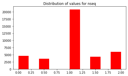
This variable take only 5 different values between 0 and 2, symmetrically distributed around 1.

`rssi`

plt.figure(figsize=(7,4))
sns.distplot(df_mess_train.rssi, bins=200, color='red')
plt.title("Distribution of values for rssi")
plt.show()

png

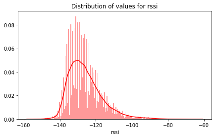
The values are distributed around -100 and -140, most around -130.

`time_ux`

plt.figure(figsize=(7,4))
sns.distplot(df_mess_train.time_ux, bins=100, kde=False, color='red')
plt.title("Distribution of values for time_ux")
plt.show()

png

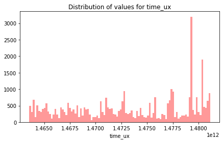
The data is evenly distributed over time, with a significant peak towards the end.

`bsid`

plt.figure(figsize=(7,4))
sns.distplot(df_mess_train.bsid, bins=100, kde=False, color='red')
plt.title("Distribution of the number of messages by bsid")
plt.show()

png

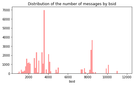
We note that some stations receive many more messages than others. This should be taken into account when analyzing the poorly represented categories.

`did`

plt.figure(figsize=(7,4))
abcisse = list((x for x in range(0,df_mess_train.did.nunique())))
plt.bar(abcisse, list(df_mess_train.groupby(['did']).messid.nunique()), width=1, color='red')
plt.title("Distribution of number of messages by device id")
plt.show()

png

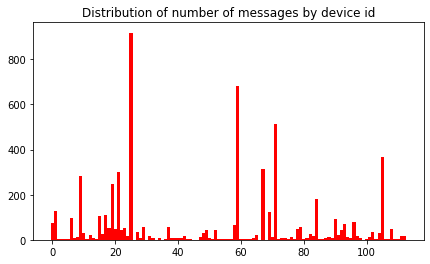
We note that the values of the device ids are also very different. Some devices emit many more messages than others. The repartition is quite similar to that of the station ids (bsid), because some devices stay near the same stations when they emit. We will also have to look at the number of messages per device_id and analyze the device_id less represented.

1.4. Correlation between variables

plt.figure(figsize=(7,5), dpi=80)
sns.heatmap(df_mess_train.corr(), cmap='PuOr', center=0, annot=True)
plt.title('Correlation matrix', fontsize=12)
plt.show()

png

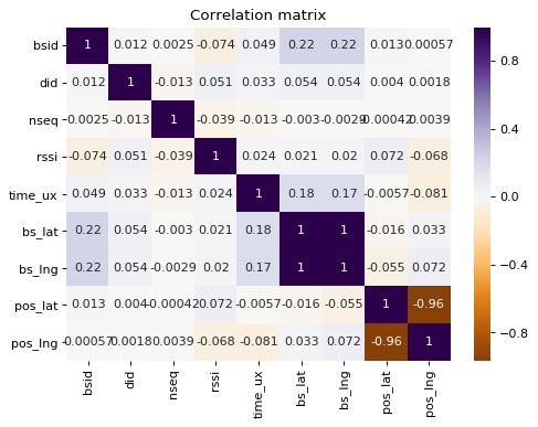
We note that there are few significant correlations between variables, with the exception of station longitude and latitude.

1.5. Detection of outliers

We will display the positions of the stations that received the messages, and the positions of the messages (the positions are the labels of the dataset):

import plotly.express as px
import plotly.graph_objects as go

fig = go.Figure()
fig.add_trace(go.Scattermapbox(lat=df_mess_train["bs_lat"], lon=df_mess_train["bs_lng"], name="Stations", 
                               marker=go.scattermapbox.Marker(size=5,color='red',opacity=0.7,)))
fig.add_trace(go.Scattermapbox(lat=df_mess_train["pos_lat"], lon=df_mess_train["pos_lng"], name="Messages", 
                               marker=go.scattermapbox.Marker(size=4,color='blue',opacity=0.7,)))

fig.update_layout(mapbox_style="open-street-map", height=400)
fig.update_layout(margin={"r":0,"t":0,"l":0,"b":0})
fig.show()

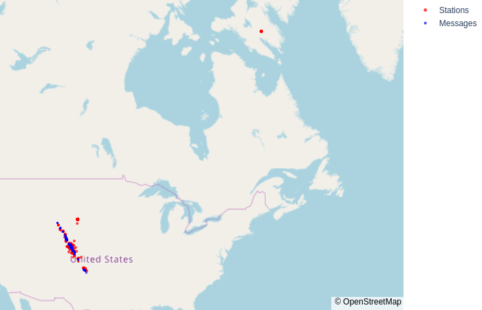
Position of the stations and messages

Some stations are far away from the others. These stations are located in the north of Canada, at a lattitude of 65 and a longitude of -70 .
All the messages are located in the same area, and surrounded by stations.

We will see if the distant stations have received messages:

df_messages_distant_stations = df_mess_train[(df_mess_train["bs_lat"] > 42) & (df_mess_train["bs_lng"] > -104)]

fig = go.Figure()
fig.add_trace(go.Scattermapbox(lat=df_messages_distant_stations["bs_lat"], lon=df_messages_distant_stations["bs_lng"], name="Stations", 
                               marker=go.scattermapbox.Marker(size=5,color='red',opacity=0.7,)))
fig.add_trace(go.Scattermapbox(lat=df_messages_distant_stations["pos_lat"], lon=df_messages_distant_stations["pos_lng"], name="Messages", 
                               marker=go.scattermapbox.Marker(size=5,color='blue',opacity=0.7,)))

fig.update_layout(mapbox_style="open-street-map", height=400)
fig.update_layout(margin={"r":0,"t":0,"l":0,"b":0})
fig.show()

Position of devices sending messages to distant stations

It is therefore clear that no message was sent at longitudes and latitudes near -70 and 65. We can consider these stations as outliers. Consequently, we deduce that the latitudes and longitudes of these stations are erroneous and a strategy to deal with these anomalies should be defined.

We list these outlier stations:

list_station_outliers = df_messages_distant_stations["bsid"].unique()
list_devices_outliers = df_messages_distant_stations["did"].unique()
list_messages_outliers = df_messages_distant_stations["messid"].unique()
messages_to_outliers = df_mess_train[df_mess_train['bsid'].isin(list_station_outliers)].groupby('bsid').count()
print("Number of outlier stations: ", len(list_station_outliers))
print("Number of devices sending messages to outlier stations:", len(list_devices_outliers))
print("Number of messages receveid by outlier stations:", messages_to_outliers['messid'].sum())
print("Represent a percentage of {:.2f}% among all the received messages".format(100*messages_to_outliers['messid'].sum() / df_mess_train.shape[0]))

Number of outlier stations:  37
Number of devices sending messages to outlier stations: 49
Number of messages receveid by outlier stations: 4567
Represent a percentage of 11.64% among all the received messages

The concerned messages received by the outliers represent a quite consequent part of the dataset.

We will check if the concerned devices have sent messages to other stations:

df_mess_to_outliers = df_mess_train[df_mess_train['messid'].isin(list_messages_outliers)]

fig = go.Figure()
fig.add_trace(go.Scattermapbox(lat=df_mess_to_outliers["bs_lat"], lon=df_mess_to_outliers["bs_lng"], name="Stations", 
                               marker=go.scattermapbox.Marker(size=6,color='red',opacity=0.7,)))
fig.add_trace(go.Scattermapbox(lat=df_mess_to_outliers["pos_lat"], lon=df_mess_to_outliers["pos_lng"], name="Messages", 
                               marker=go.scattermapbox.Marker(size=6,color='blue',opacity=0.7,)))

fig.update_layout(mapbox_style="open-street-map", height=400)
fig.update_layout(margin={"r":0,"t":0,"l":0,"b":0})
fig.show()

Position of the stations receiving the same messages as the outliers stations.

We see that meanwhile an important number of messages are concerned by the outliers, there alse are an important number of other stations that have received the same messages, and they can cover the reception of those messages.

So we define 3 options:

We will considers the others stations will be enough to receive the messages, so we delete the outliers
We will relocate the outlier stations on the map, to keep the number of station we have in our dataset. We will relocate the outliers by doing an average with the neighbour stations.
We will improve the relocate by relocating the outliers with a random forest, to make a regression to predict the latitude and longitude of the stations.

We will implement the third option. A table summarizes the scores obtained with each option at the end.

1.6. Relocation of outliers by random forest

We are going to implement another way to replace the points, by random forest:

1.6.1. Prepare the datasets

We prepare the datasets for the prediction, mainly by one hot encoding the message ids:

# List the concerned messages
listOfMessIds = df_mess_to_outliers["messid"].unique()
listOfMessIds = ["mess_"+str(code) for code in listOfMessIds]

# One hot encode the message ids
ohe = OneHotEncoder()
X_messid = ohe.fit_transform(df_mess_to_outliers[['messid']]).toarray()

df_messid_train = pd.DataFrame(X_messid, columns = listOfMessIds)
df_mess_to_outliers[listOfMessIds] = df_messid_train
df_mess_to_outliers.fillna(0, inplace=True)


## Train set: the messages received by stations correctly located.
train = df_mess_to_outliers[~df_mess_to_outliers["bsid"].isin(list_station_outliers)]
y_lat = train['bs_lat']
y_lng = train['bs_lng']
X = train.drop(["bs_lat","bs_lng", "messid"], axis=1)
X_train, X_test, y_lat_train, y_lat_test, y_lng_train, y_lng_test = train_test_split(X, y_lat, y_lng, test_size = 0.2, random_state=261)

## Prediction set: the messages received by outlier stations
pred  = df_mess_to_outliers[df_mess_to_outliers["bsid"].isin(list_station_outliers)]
X_pred = pred.drop(["bs_lat","bs_lng", "messid"], axis=1)

1.6.2. Train the model

The model is a simple random forest, with 1000 estimators and default parameters:

clf_lat = RandomForestRegressor(n_estimators=1000, n_jobs=-1, random_state=261)
clf_lat.fit(X_train, y_lat_train)

clf_lng = RandomForestRegressor(n_estimators=1000, n_jobs=-1, random_state=261)
clf_lng.fit(X_train, y_lng_train)

RandomForestRegressor(bootstrap=True, criterion='mse', max_depth=None,
                      max_features='auto', max_leaf_nodes=None,
                      min_impurity_decrease=0.0, min_impurity_split=None,
                      min_samples_leaf=1, min_samples_split=2,
                      min_weight_fraction_leaf=0.0, n_estimators=1000,
                      n_jobs=-1, oob_score=False, random_state=261, verbose=0,
                      warm_start=False)

score_lat = clf_lat.score(X_test, y_lat_test)
score_lng = clf_lng.score(X_test, y_lng_test)
print("Score for latitude:  {:.4f}".format(score_lat))
print("Score for longitude: {:.4f}".format(score_lng))

Score for latitude:  0.8913
Score for longitude: 0.8441

The score is quite good for our need. We will use this model.

1.6.3. Make the predictions and integrate them in the initial dataset

# We compute the predictions
X_pred["bs_lat_new"] = clf_lat.predict(X_pred)
X_pred["bs_lng_new"] = clf_lng.predict(X_pred)

# We integrate them to the initial dataset
df_mess_train = df_mess_train.merge(X_pred, how="left", left_index=True, right_index=True)
df_mess_train["bs_lat"] = df_mess_train.apply(lambda x: x["bs_lat_new"] if not pd.isna(x["bs_lat_new"]) else x["bs_lat"], axis=1)
df_mess_train["bs_lng"] = df_mess_train.apply(lambda x: x["bs_lng_new"] if not pd.isna(x["bs_lng_new"]) else x["bs_lng"], axis=1)
df_mess_train.drop(["bs_lat_new", "bs_lng_new"], axis=1, inplace=True)
df_mess_train.tail(5)

	messid	bsid	did	nseq	rssi	time_ux	bs_lat	bs_lng	pos_lat	pos_lng	bs_lat_new	bs_lng_new
0	573bf1d9864fce1a9af8c5c9	2841	473335.0	0.5	-121.500000	1.463546e+12	39.617794	-104.954917	39.606690	-104.958490	NaN	NaN
1	573bf1d9864fce1a9af8c5c9	3526	473335.0	2.0	-125.000000	1.463546e+12	39.677251	-104.952721	39.606690	-104.958490	NaN	NaN
2	573bf3533e952e19126b256a	2605	473335.0	1.0	-134.000000	1.463547e+12	39.612745	-105.008827	39.637741	-104.958554	NaN	NaN
3	573c0cd0f0fe6e735a699b93	2610	473953.0	2.0	-132.000000	1.463553e+12	39.797969	-105.073460	39.730417	-104.968940	NaN	NaN
4	573c0cd0f0fe6e735a699b93	3574	473953.0	1.0	-120.000000	1.463553e+12	39.723151	-104.956216	39.730417	-104.968940	NaN	NaN
...	...	...	...	...	...	...	...	...	...	...	...	...
39245	5848672e12f14360d7942374	3410	476257.0	1.0	-128.000000	1.481140e+12	39.777690	-105.002424	39.773264	-105.014052	NaN	NaN
39246	5848672e12f14360d7942374	8352	476257.0	0.0	-121.000000	1.481140e+12	39.761633	-105.025753	39.773264	-105.014052	NaN	NaN
39247	5848672e12f14360d7942374	8397	476257.0	2.0	-126.000000	1.481140e+12	39.759396	-105.001415	39.773264	-105.014052	NaN	NaN
39248	58487473e541cd0e133cca72	3051	476593.0	1.0	-131.333333	1.481143e+12	39.898872	-105.153832	39.908186	-105.168297	NaN	NaN
39249	58487473e541cd0e133cca72	7692	476593.0	1.5	-135.000000	1.481143e+12	39.928436	-105.172719	39.908186	-105.168297	NaN	NaN

39250 rows × 12 columns

1.6.4. Display the relocated stations

Here is the result of the relocated stations (in green on the map):

fig = go.Figure()
mask = df_mess_train3["bsid"].isin(list_station_outliers)
fig.add_trace(go.Scattermapbox(lat=df_mess_train3[~mask]["bs_lat"], lon=df_mess_train3[~mask]["bs_lng"], name="Stations", 
                               marker=go.scattermapbox.Marker(size=7,color='red',opacity=0.7,)))
fig.add_trace(go.Scattermapbox(lat=df_mess_train3[mask]["bs_lat_new"], lon=df_mess_train3[mask]["bs_lng_new"], name="Stations relocated", 
                               marker=go.scattermapbox.Marker(size=7,color='green',opacity=0.7,)))
fig.add_trace(go.Scattermapbox(lat=df_mess_train3["pos_lat"], lon=df_mess_train3["pos_lng"], name="Messages", 
                               marker=go.scattermapbox.Marker(size=7,color='blue',opacity=0.7,)))

fig.update_layout(mapbox_style="open-street-map", height=400)
fig.update_layout(margin={"r":0,"t":0,"l":0,"b":0})
fig.show()

Position of the relocated stations (in green)

We isolate one message, and display the location of all the stations that have received it. The relocated station (in green) was badly located in the north of Canada before, and is now in the town downtown area of Denver:

df_mess_to_outliers4 = df_mess_train3[df_mess_train3["messid"] == "57617e1ef0fe6e0c9fd6eb06"]
df_mess_to_outliers4

fig = go.Figure()
mask = df_mess_to_outliers4["bsid"].isin(list_station_outliers)
fig.add_trace(go.Scattermapbox(lat=df_mess_to_outliers4[~mask]["bs_lat"], lon=df_mess_to_outliers4[~mask]["bs_lng"], name="Stations", 
                               marker=go.scattermapbox.Marker(size=7,color='red',opacity=0.7,)))
fig.add_trace(go.Scattermapbox(lat=df_mess_to_outliers4[mask]["bs_lat_new"], lon=df_mess_to_outliers4[mask]["bs_lng_new"], name="Stations relocated", 
                               marker=go.scattermapbox.Marker(size=7,color='green',opacity=0.7,)))
fig.add_trace(go.Scattermapbox(lat=df_mess_to_outliers4["pos_lat"], lon=df_mess_to_outliers4["pos_lng"], name="Messages", 
                               marker=go.scattermapbox.Marker(size=7,color='blue',opacity=0.7,)))

fig.update_layout(mapbox_style="open-street-map", height=400)
fig.update_layout(margin={"r":0,"t":0,"l":0,"b":0})
fig.show()

Position of the relocated stations for a message in particular.

1.7. Detection of less represented classes

We will find the stations that process few messages to potentially remove them from the training set in order to keep only the most representative stations and thus have the most reliable categories to make predictions.

# We look base stations that aren't getting a lot of messages
count_basestation = df_mess_train.groupby('bsid').count()
count_basestation = count_basestation['messid']
mes_limit = 500 # Limit

plt.figure(figsize=(8,6))
count_basestation_cum = count_basestation.sort_values(ascending=True).cumsum()
plt.plot(count_basestation_cum.values)

x = [0, count_basestation_cum.count()]
y = [mes_limit, mes_limit]
plt.plot(x, y, color ='black')
plt.title("Cumulative sum of messages according to the {} stations \n".format(df_mess_train.bsid.nunique()), size=12)
plt.show()

png

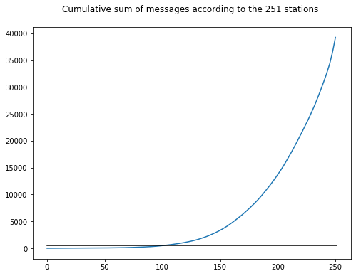
print("Number of stations under a cumulative sum of {:d} : {:d}".format(mes_limit, (count_basestation_cum < mes_limit).sum()))

Number of stations under a cumulative sum of 500 : 101

We can therefore see that there are 95 stations that receive few messages but that the others receive significantly more.
We decide to remove the stations receiving few messages:

# Removing the corresponding messages
bsid_to_remove = count_basestation_cum[count_basestation_cum < mes_limit].index.values
df_mess_train = df_mess_train[~df_mess_train.bsid.isin(bsid_to_remove)]

# Reset index
df_mess_train = df_mess_train.reset_index().drop(columns=['index'])
n_train = df_mess_train.shape[0]

2. Features engineering

2.1. One hot encoding of the station ids

List the remaining stations:

listOfBs = df_mess_train.bsid.unique()
listNameBs = ["bs"+str(code) for code in listOfBs]
print("Number of remaining stations : ", len(listOfBs))

Number of remaining stations :  150

One hot encoding:

ohe = OneHotEncoder()
X_bsid = ohe.fit_transform(df_mess_train[['bsid']]).toarray()
df_bsid_train = pd.DataFrame(X_bsid[:n_train,:], columns = listNameBs)

# We add the columns from our encoder to our training dataset
df_mess_train[listNameBs] = df_bsid_train

2.2. Prepare intermediary dataframes

We keep the did (device id) associated with each message, to be able to use it in the final dataset.

listOfDid = df_mess_train.did.unique()
listNameDid = ["did"+str(int(i)) for i in listOfDid]
print("Number of remaining devices: ", len(listOfDid))

Number of remaining devices:  112

df_grouped_train_did = df_mess_train.groupby(['messid', 'did']).count().reset_index(level=['did'])["did"]

Group the dataset by different variables

We create different intermediary datasets, that will be useful to compute the final features matrix:

# Group the dataset by `messid`
df_grouped_train = df_mess_train.groupby(['messid'])

# Group of `bsid` by `messid`
df_bsid_grouped_train = df_grouped_train.sum()[listNameBs]

# DeviceID of MessID
did_grouped_train = df_grouped_train.mean()['did'].values

# Average RSSI by MessID
rssi_grouped_train = df_grouped_train.mean()['rssi'].values

# Average time_ux of message reception
time_ux_grouped_train = df_grouped_train.mean()['time_ux'].values

# Average lat/long of base stations that received the message
lat_grouped_train = df_grouped_train.mean()['bs_lat'].values
lng_grouped_train = df_grouped_train.mean()['bs_lng'].values

# Average lat/long of base stations weighted by other variables
# Weighted by the RSSI, the strength of the received signal
lat_rssi_grouped_train = np.array([np.average(elmt['bs_lat'], weights=elmt['rssi']) for key, elmt in df_grouped_train])
lng_rssi_grouped_train = np.array([np.average(elmt['bs_lng'], weights=elmt['rssi']) for key, elmt in df_grouped_train])

# Weighted by time_ux
time_ux_lat_grouped_train = np.array([np.average(elmt['bs_lat'], weights=elmt['time_ux']) for key, elmt in df_grouped_train])
time_ux_lng_grouped_train = np.array([np.average(elmt['bs_lng'], weights=elmt['time_ux']) for key, elmt in df_grouped_train])

# Weighted by nseq
nseq_lat_grouped_train = np.array([np.average(elmt['bs_lat'], weights=elmt['nseq']+1) for key, elmt in df_grouped_train])
nseq_lng_grouped_train = np.array([np.average(elmt['bs_lng'], weights=elmt['nseq']+1) for key, elmt in df_grouped_train])

# Average lat/long by labels (which means lat/long of the devices)
pos_lat_grouped_train = df_grouped_train.mean()['pos_lat'].values
pos_lng_grouped_train = df_grouped_train.mean()['pos_lng'].values

2.3. Features selection

We build a dataframe based on the dataset we just computed. We choose to average the different variables for the same message.

# We create the dataframe, with the features we want to add
df_train = pd.DataFrame()
df_train["did"] = df_grouped_train_did
df_train['mean_rssi'] = rssi_grouped_train
df_train['mean_lat'] = lat_grouped_train
df_train['mean_lng'] = lng_grouped_train
df_train['mean_lat_rssi'] = lat_rssi_grouped_train
df_train['mean_lng_rssi'] = lng_rssi_grouped_train
df_train['mean_time_ux'] = time_ux_grouped_train
df_train[listNameBs] = df_bsid_grouped_train
df_train['pos_lat'] = pos_lat_grouped_train
df_train['pos_lng'] = pos_lng_grouped_train
df_train

	did	mean_rssi	mean_lat	mean_lng	mean_lat_rssi	mean_lng_rssi	mean_time_ux	bs2841	bs3526	bs2605	...	bs2707	bs2943	bs1092	bs3848	bs2803	bs3630	bs2800	bs1854	pos_lat	pos_lng
messid
573bf1d9864fce1a9af8c5c9	473335.0	-123.250000	39.647522	-104.953819	39.647945	-104.953803	1.463546e+12	0.0	0.0	0.0	...	0.0	0.0	0.0	0.0	0.0	0.0	0.0	0.0	39.606690	-104.958490
573bf3533e952e19126b256a	473335.0	-134.000000	39.612745	-105.008827	39.612745	-105.008827	1.463547e+12	0.0	0.0	0.0	...	0.0	0.0	0.0	0.0	0.0	0.0	0.0	0.0	39.637741	-104.958554
573c0cd0f0fe6e735a699b93	473953.0	-117.333333	39.751055	-105.001109	39.753734	-105.005136	1.463553e+12	0.0	0.0	0.0	...	0.0	0.0	0.0	0.0	0.0	0.0	0.0	0.0	39.730417	-104.968940
573c1272f0fe6e735a6cb8bd	476512.0	-127.416667	39.616885	-105.030503	39.614550	-105.030671	1.463555e+12	0.0	0.0	0.0	...	0.0	0.0	0.0	0.0	0.0	0.0	0.0	0.0	39.693102	-105.006995
573c8ea8864fce1a9a5fbf7a	476286.0	-125.996032	39.778865	-105.033121	39.779871	-105.033005	1.463586e+12	0.0	1.0	0.0	...	0.0	0.0	0.0	0.0	1.0	0.0	0.0	0.0	39.758167	-105.051016
...	...	...	...	...	...	...	...	...	...	...	...	...	...	...	...	...	...	...	...	...	...
5848551912f14360d786ede6	476207.0	-125.500000	39.769873	-105.001500	39.769929	-105.001249	1.481135e+12	0.0	0.0	0.0	...	0.0	0.0	0.0	0.0	0.0	0.0	0.0	0.0	39.764915	-105.003985
58485a25e541cd0e1329b8d6	476512.0	-129.566667	39.678859	-105.024327	39.679685	-105.025102	1.481137e+12	0.0	0.0	0.0	...	0.0	0.0	0.0	0.0	0.0	0.0	0.0	0.0	39.658804	-105.008299
58485bd412f14360d78bebdb	476207.0	-128.383333	39.670843	-104.935855	39.676092	-104.939543	1.481137e+12	0.0	0.0	0.0	...	0.0	0.0	0.0	0.0	1.0	1.0	0.0	1.0	39.778872	-105.019285
5848672e12f14360d7942374	476257.0	-123.800000	39.757494	-105.012860	39.756802	-105.012642	1.481140e+12	0.0	0.0	0.0	...	0.0	0.0	0.0	0.0	0.0	0.0	0.0	0.0	39.773264	-105.014052
58487473e541cd0e133cca72	476593.0	-133.166667	39.913654	-105.163275	39.913858	-105.163405	1.481143e+12	0.0	0.0	0.0	...	0.0	0.0	0.0	0.0	0.0	0.0	0.0	0.0	39.908186	-105.168297

5975 rows × 159 columns

We will see which features are most important on a RandomForestRegressor model. This will allow us to fine-tune the selection of our variables and improve the training performance of our model.

X_train = df_train.iloc[:,:-2]
y_lat_train = df_train['pos_lat']
y_lng_train = df_train['pos_lng']

We fit the RandomForest:

clf_lat = RandomForestRegressor(n_estimators=1000, n_jobs=-1, random_state=261)
clf_lat.fit(X_train, y_lat_train)

clf_lng = RandomForestRegressor(n_estimators=1000, n_jobs=-1, random_state=261)
clf_lng.fit(X_train, y_lng_train)

RandomForestRegressor(bootstrap=True, criterion='mse', max_depth=None,
                      max_features='auto', max_leaf_nodes=None,
                      min_impurity_decrease=0.0, min_impurity_split=None,
                      min_samples_leaf=1, min_samples_split=2,
                      min_weight_fraction_leaf=0.0, n_estimators=1000,
                      n_jobs=-1, oob_score=False, random_state=261, verbose=0,
                      warm_start=False)

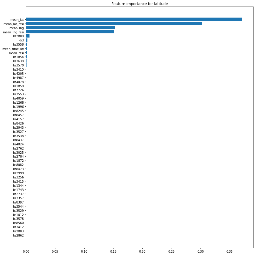
Calculation of feature importance for latitude and longitude:

dict_feature_importance_lat = {'feature': X_train.columns.values, 
                               'importance': clf_lat.feature_importances_}
feature_importances_lat = pd.DataFrame(data=dict_feature_importance_lat).sort_values('importance', ascending=False)

dict_feature_importance_lng = {'feature': X_train.columns.values, 
                               'importance': clf_lng.feature_importances_}
feature_importances_lng = pd.DataFrame(data=dict_feature_importance_lng).sort_values('importance', ascending=False)

We set a treshold to consider the features as interesting ones:

importance_treshold = 0.000025

Result for the prediction of the latitude:

mask_lat = feature_importances_lat['importance'] > importance_treshold
plt.figure(figsize=(12,12))
plt.barh(feature_importances_lat['feature'][mask_lat], feature_importances_lat['importance'][mask_lat])  
plt.title('Feature importance for latitude')
plt.tight_layout()
plt.gca().invert_yaxis()
plt.show()

png

We do the same for the longitude:

mask_lng = feature_importances_lng['importance'] > importance_treshold
plt.figure(figsize=(12,12))
plt.barh(feature_importances_lng['feature'][mask_lng], feature_importances_lng['importance'][mask_lng])      
plt.title('Feature importance for longitude')
plt.tight_layout()
plt.gca().invert_yaxis()
plt.show()

png

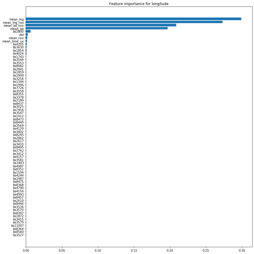
It is therefore quite clear that only a few variables are of overriding importance compared to the others. We are therefore going to remove from our training set the features whose importance is low, i.e. at the threshold of 0.000025.

mask_lat = feature_importances_lat['importance'] > importance_treshold
mask_lng = feature_importances_lng['importance'] > importance_treshold

# We use set() to have the intersection of our ensembles
indexes_to_remove = list(set(feature_importances_lat['feature'][np.logical_not(mask_lat)]
         ).intersection(set(feature_importances_lng['feature'][np.logical_not(mask_lng)])))

print("{:d} features have an importance lower than {:.6f}.".format(len(indexes_to_remove), importance_treshold))
X_train = X_train.drop(indexes_to_remove, axis=1)

75 features have an importance lower than 0.000025.

3. Models

We define functions to evaluate our results (those functions were given):

# Evaluation function of our results
def vincenty_vec(vec_coord):
    vin_vec_dist = np.zeros(vec_coord.shape[0])
    if vec_coord.shape[1] !=  4:
        print('ERROR: Bad number of columns (shall be = 4)')
    else:
        vin_vec_dist = [vincenty(vec_coord[m,0:2],vec_coord[m,2:]).meters for m in range(vec_coord.shape[0])]
    return vin_vec_dist


# Evaluate distance error for each predicted point
def Eval_geoloc(y_train_lat , y_train_lng, y_pred_lat, y_pred_lng):
    vec_coord = np.array([y_train_lat , y_train_lng, y_pred_lat, y_pred_lng])
    err_vec = vincenty_vec(np.transpose(vec_coord))
    return err_vec

# Display of cumulative error
def grap_error(err_vec):
    values, base = np.histogram(err_vec, bins=50000)
    cumulative = np.cumsum(values) 
    plt.figure()
    plt.plot(base[:-1]/1000, cumulative / np.float(np.sum(values))  * 100.0, c='blue')
    plt.grid()
    plt.xlabel('Distance Error (km)')
    plt.ylabel('Cum proba (%)'); plt.axis([0, 30, 0, 100]) 
    plt.title('Error Cumulative Probability')
    plt.legend( ["Opt LLR", "LLR 95", "LLR 99"])
    plt.show()

3.1. Model `RandomForestRegressor`

We will now optimize our RandomForest algorithm. To do this, we will look at the depth of the max_depth tree, the proportion of features to be considered at each branch separation max_features, and the number of n_estimators.

# We prepare our dataframes to perform a gridSearch
Xtrain_cv, Xtest_cv, y_lat_train_cv, y_lat_test_cv, y_lng_train_cv, y_lng_test_cv = \
    train_test_split(X_train, y_lat_train, y_lng_train, test_size=0.2, random_state=261)

We perform a manual Grid Search, rather than using prebuilt function, because it is more adapted to optimize our two models (for latitude and longitude) together.

# Manual Gridsearch 
list_max_depth = [20, 25, 30, 35, 40, 45, 50]
list_max_features = [0.5, 0.6, 0.7, 0.8, 0.9, None]
list_n_estimators = [50, 100, 200]
  
err80 = 10000
list_result =[]
for max_depth in list_max_depth:
    print('Step max_depth : ', str(max_depth))
    for max_features in list_max_features:
        for n_estimators in list_n_estimators:
            clf_rf_lat = RandomForestRegressor(n_estimators = n_estimators, max_depth=max_depth,
                                               max_features = max_features, n_jobs=-1)
            clf_rf_lat.fit(Xtrain_cv, y_lat_train_cv)
            y_pred_lat = clf_rf_lat.predict(Xtest_cv) 

            clf_rf_lng = RandomForestRegressor(n_estimators = n_estimators, max_depth=max_depth,
                                               max_features = max_features,n_jobs=-1)
            clf_rf_lng.fit(Xtrain_cv, y_lng_train_cv)
            y_pred_lng = clf_rf_lng.predict(Xtest_cv)

            err_vec = Eval_geoloc(y_lat_test_cv , y_lng_test_cv, y_pred_lat, y_pred_lng)
            perc = np.percentile(err_vec, 80)
            list_result.append((max_depth,max_features,n_estimators, perc))
            if perc < err80: # minimum error distance for 80% of the observations
                err80 = perc
                best_max_depth = max_depth
                best_max_features = max_features
                best_n_estimators = n_estimators    

print('--- Final results ---')
print('best_max_depth', best_max_depth) 
print('best_max_features', best_max_features)
print('best_n_estimators', best_n_estimators)
print('err80', err80)

--- Final results ---
best_max_depth 40
best_max_features 0.6
best_n_estimators 100
err80 2544.882038827355

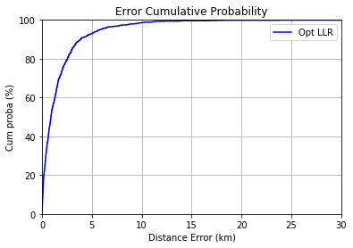
We train our RandomForest model on 80% of the train set and validate it on the remaining 20%. The model is trained with the best hyperparameters we just found.

clf_rf_lat = RandomForestRegressor(n_estimators = best_n_estimators, 
                                   max_features = best_max_features, 
                                   max_depth = best_max_depth, n_jobs=-1)
clf_rf_lat.fit(Xtrain_cv, y_lat_train_cv)
y_pred_lat = clf_rf_lat.predict(Xtest_cv) 

clf_rf_lng = RandomForestRegressor(n_estimators = best_n_estimators, 
                                   max_features = best_max_features, 
                                   max_depth = best_max_depth, n_jobs=-1)
clf_rf_lng.fit(Xtrain_cv, y_lng_train_cv)
y_pred_lng = clf_rf_lng.predict(Xtest_cv)

err_vec = Eval_geoloc(y_lat_test_cv , y_lng_test_cv, y_pred_lat, y_pred_lng)
print("Cumulative distance error at 80% : {} \n" .format((np.percentile(err_vec, 80))))

grap_error(err_vec)

Cumulative distance error at 80% : 2679.0497470797027

png

3.2. Model `ExtraTreesRegressor`

We test another ensemble algorithm with a new Grid Search.

# Manual Gridsearch
list_max_depth = [20, 25, 30, 35, 40, 45, 50, 55, 60]
list_max_features = [0.5, 0.6, 0.7, 0.8, 0.9, None]
list_n_estimators = [50, 100, 200]
  
err80 = 10000
list_result =[]
for max_depth in list_max_depth:
    print('Step max_depth : '+str(max_depth))
    for max_features in list_max_features:
        for n_estimators in list_n_estimators:
            clf_et_lat = ExtraTreesRegressor(n_estimators = n_estimators, max_depth=max_depth,
                                               max_features = max_features, n_jobs=-1)
            clf_et_lat.fit(Xtrain_cv, y_lat_train_cv)
            y_pred_lat = clf_et_lat.predict(Xtest_cv) 

            clf_et_lng = ExtraTreesRegressor(n_estimators = n_estimators, max_depth=max_depth,
                                               max_features = max_features,n_jobs=-1)
            clf_et_lng.fit(Xtrain_cv, y_lng_train_cv)
            y_pred_lng = clf_et_lng.predict(Xtest_cv)

            err_vec = Eval_geoloc(y_lat_test_cv , y_lng_test_cv, y_pred_lat, y_pred_lng)
            perc = np.percentile(err_vec, 80)
            list_result.append((max_depth,max_features,n_estimators, perc))
            if perc < err80: # minimum error distance for 80% of the observations
                err80 = perc
                best_max_depth = max_depth
                best_max_features = max_features
                best_n_estimators = n_estimators    

print('--- Final results ---')               
print('best_max_depth', best_max_depth) 
print('best_max_features', best_max_features)
print('best_n_estimators', best_n_estimators)
print('err80', err80)

--- Final results ---
best_max_depth 30
best_max_features 0.9
best_n_estimators 100
err80 2442.480237084153

We then train and validate the model:

clf_lat = ExtraTreesRegressor(n_estimators=best_n_estimators, max_features=best_max_features, 
                              max_depth=best_max_depth, n_jobs=-1)
clf_lat.fit(Xtrain_cv, y_lat_train_cv)
y_pred_lat = clf_lat.predict(Xtest_cv)
clf_lng = ExtraTreesRegressor(n_estimators=best_n_estimators, max_features=best_max_features, 
                              max_depth=best_max_depth, n_jobs=-1)
clf_lng.fit(Xtrain_cv, y_lng_train_cv)
y_pred_lng = clf_lng.predict(Xtest_cv)

err_vec = Eval_geoloc(y_lat_test_cv , y_lng_test_cv, y_pred_lat, y_pred_lng)
print("Cumulative distance error at 80% : {} \n" .format((np.percentile(err_vec, 80))))

grap_error(err_vec)

Cumulative distance error at 80% : 2544.639183263528

png

The scores are very close, but a little better with the ExtraTreeRegressor.

4. Cross validation with leave one device out

In this part we will implement a cross validation, of type leave one out. This is necessary to have a more realistic prediction score, when we will use our model with never seen devices, in production. To do so, we will train the model on the whole training set deprived of all the messages of one device (a different device at each iteration).

We will perform the cross validation on both models because their scores were close.

4.1. Definition of the parameters for the cross validation

We create the groups, defined by the device ids.

from sklearn.model_selection import LeaveOneGroupOut
groups = np.array(X_train["did"].tolist())
logo = LeaveOneGroupOut()
logo.get_n_splits(X_train, y_lat_train, groups)

There are 112 folds.

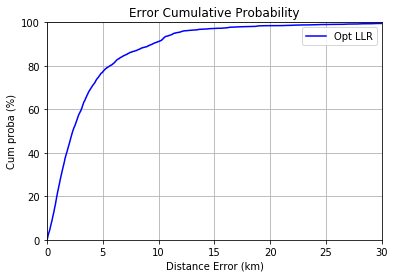
4.2. Cross validation with the model `RandomForestRegressor`

We perform the cross validation for the latitude and longitude:

cv_lat = logo.split(X_train, y_lat_train, groups)
y_pred_lat = cross_val_predict(clf_rf_lat, X_train, y_lat_train, cv=cv_lat)

cv_lng = logo.split(X_train, y_lng_train, groups)
y_pred_lng = cross_val_predict(clf_rf_lng, X_train, y_lng_train, cv=cv_lng)

We display the error curve:

err_vec = Eval_geoloc(y_lat_train , y_lng_train, y_pred_lat, y_pred_lng)
print("Cumulative distance error at 80% : {} \n" .format((np.percentile(err_vec, 80))))

grap_error(err_vec)

Cumulative distance error at 80% : 5625.2904721246705

png

4.3. Cross validation with the model `ExtraTreesRegressor`

We do the same with this model:

cv_lat = logo.split(X_train, y_lat_train, groups)
y_pred_lat = cross_val_predict(clf_lat, X_train, y_lat_train, cv=cv_lat)

cv_lng = logo.split(X_train, y_lng_train, groups)
y_pred_lng = cross_val_predict(clf_lng, X_train, y_lng_train, cv=cv_lng)

err_vec = Eval_geoloc(y_lat_train , y_lng_train, y_pred_lat, y_pred_lng)
print("Cumulative distance error at 80% : {} \n" .format((np.percentile(err_vec, 80))))

grap_error(err_vec)

Cumulative distance error at 80% : 5525.364650779721

png

The score is much worse in cross validation by leave one device out, because the predictions are made on devices on which the model has not been trained. This is a more realistic score.

5. Conclusion

Summary of the scores obtained with the different models and pre-processing:

	Outliers deleted	Outliers replaced
RandomForestRegressor	2679	2645
ExtraTreesRegressor	2669	2544
RandomForestRegressor cross-validation	6271	5625
ExtraTreesRegressor cross-validation	5276	5525

Scores representing a prediction error in meters, the lower the better.
The ExtraTreesRegressor give better results. The cross-validation gives better results when the outliers are simply deleted.

This lab shows how to explore a dataset before applying a model, with sometimes important operations to apply to clean and adjust our data. Then, we see the importance of a cross-validation by leave-one-out to obtain a score more realist for production purposes.

You can see the complete code and project explanations on the GitHub repository of the project.

Illustration photo by Pixabay

Xavier B.

My name is Xavier. I love data science.
Feel free to contact me!

Predict IoT device geolocation

Imports

1. Load and explore data

1.1. Data loading

1.2. Data description

Table messages

Table positions

Tables messages and positions joined

1.3. Value distribution

`nseq`

`rssi`

`time_ux`

`bsid`

`did`

1.4. Correlation between variables

1.5. Detection of outliers

1.6. Relocation of outliers by random forest

1.6.1. Prepare the datasets

1.6.2. Train the model

1.6.3. Make the predictions and integrate them in the initial dataset

1.6.4. Display the relocated stations

1.7. Detection of less represented classes

2. Features engineering

2.1. One hot encoding of the station ids

2.2. Prepare intermediary dataframes

Group the dataset by different variables

2.3. Features selection

3. Models

3.1. Model `RandomForestRegressor`

3.2. Model `ExtraTreesRegressor`

4. Cross validation with leave one device out

4.1. Definition of the parameters for the cross validation

4.2. Cross validation with the model `RandomForestRegressor`

4.3. Cross validation with the model `ExtraTreesRegressor`

5. Conclusion

Xavier B.

Recent posts

Predict IoT device geolocation

Imports

1. Load and explore data

1.1. Data loading

1.2. Data description

Table messages

Table positions

Tables messages and positions joined

1.3. Value distribution

nseq

rssi

time_ux

bsid

did

1.4. Correlation between variables

1.5. Detection of outliers

1.6. Relocation of outliers by random forest

1.6.1. Prepare the datasets

1.6.2. Train the model

1.6.3. Make the predictions and integrate them in the initial dataset

1.6.4. Display the relocated stations

1.7. Detection of less represented classes

2. Features engineering

2.1. One hot encoding of the station ids

2.2. Prepare intermediary dataframes

Group the dataset by different variables

2.3. Features selection

3. Models

3.1. Model RandomForestRegressor

3.2. Model ExtraTreesRegressor

4. Cross validation with leave one device out

4.1. Definition of the parameters for the cross validation

4.2. Cross validation with the model RandomForestRegressor

4.3. Cross validation with the model ExtraTreesRegressor

5. Conclusion

Xavier B.

Recent posts

`nseq`

`rssi`

`time_ux`

`bsid`

`did`

3.1. Model `RandomForestRegressor`

3.2. Model `ExtraTreesRegressor`

4.2. Cross validation with the model `RandomForestRegressor`

4.3. Cross validation with the model `ExtraTreesRegressor`